Find a Hardware Injection: Step 3

This tutorial will pick up where step 2 left off. If you haven't already completed step 2, you may want to do that first.

Compute the matched-filter output

OK, here's the big moment. We're going to multiply the data by the template, and weight by the PSD.

integrand = data_fft*np.ma.conjugate(temp)/Pxx

Now we need to integrate over the frequency bins to compute the SNR. After accounting for different time-off sets between the template and the data, this turns out to be equivalent to transforming the result back to the time domain with an inverse Fourier Transform (IFFT). Since we used the "real" FFT to get into the frequency domain, we'll need to zero-pad before taking the IFFT.

num_zeros = len(inj_data) - len(data_fft)
padded_int = np.append( integrand, np.zeros(num_zeros) )
z = 4*np.fft.ifft(padded_int)

Compute the Normalization

The quantity σ represents the exptectation value for the matched filter output |z| when there is no signal present in the data. We can calculate σ without the data, using only the template and the PSD estimate

kernal =  (np.abs(temp))**2 / Pxx
df = psd_freq[1] - psd_freq[0]
sig_sqr = 4*kernal.sum()*df
sigma = np.sqrt(sig_sqr)

The template calculated in template.py has an amplitude normalized to 1 Mpc. This allows us to calculate the SNR we expect for a signal from 25 Mpc based on σ:

expected_SNR = sigma / 25

Compute the SNR

To transform the data to the Fourier domain, we used a window function to reduce edge effects. To get a correct value for SNR, we'll have to invert the window now.

inv_win = (1.0 / window)

The beginning and end of the matched filter output are contaminated by edge effects, so we'll set the first and last 20 seconds to zero to remove those times from the analysis:

inv_win[:20*4096] = 0
inv_win[-20*4096:] = 0

Finally, we are ready to calculate the SNR, labeled ρ:

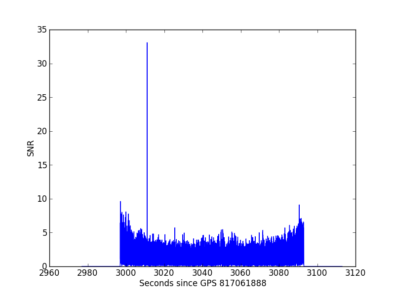
rho = abs(z) / sigma * inv_win

Rho is now a function of time, where each time corresponds to the time off-set between the filter and the data.

Output the results

# -- Plot rho as a function of time
plt.figure()
plt.plot(inj_time[::8]-time[0], rho[::8])
plt.xlabel("Seconds since GPS {0:.0f}".format(time[0]) )
plt.ylabel("SNR")

#-- Find which time off-set gives maximum value of SNR
snr = rho.max()
found_time = inj_time[ np.where(rho == snr) ]

# -- Report the results
print "\n  --- Printing Results ---"
print "Expected to find SNR {0:.1f}".format(expected_SNR)
print "Recovered SNR {0:.1f}".format(rho.max())
print "Recovered time GPS {0:.1f}".format( found_time[0] )

It looks like the injection occurs around 3011 seconds after the start of the file, which corresponds to GPS 817064899. That's the same time we saw in the injection log file, and indicates the merger time of this injection. If you run this code, you should find an SNR of 33.8.

You made it!

That's the end of this tutorial. If you like, you can look at other available tutorials.